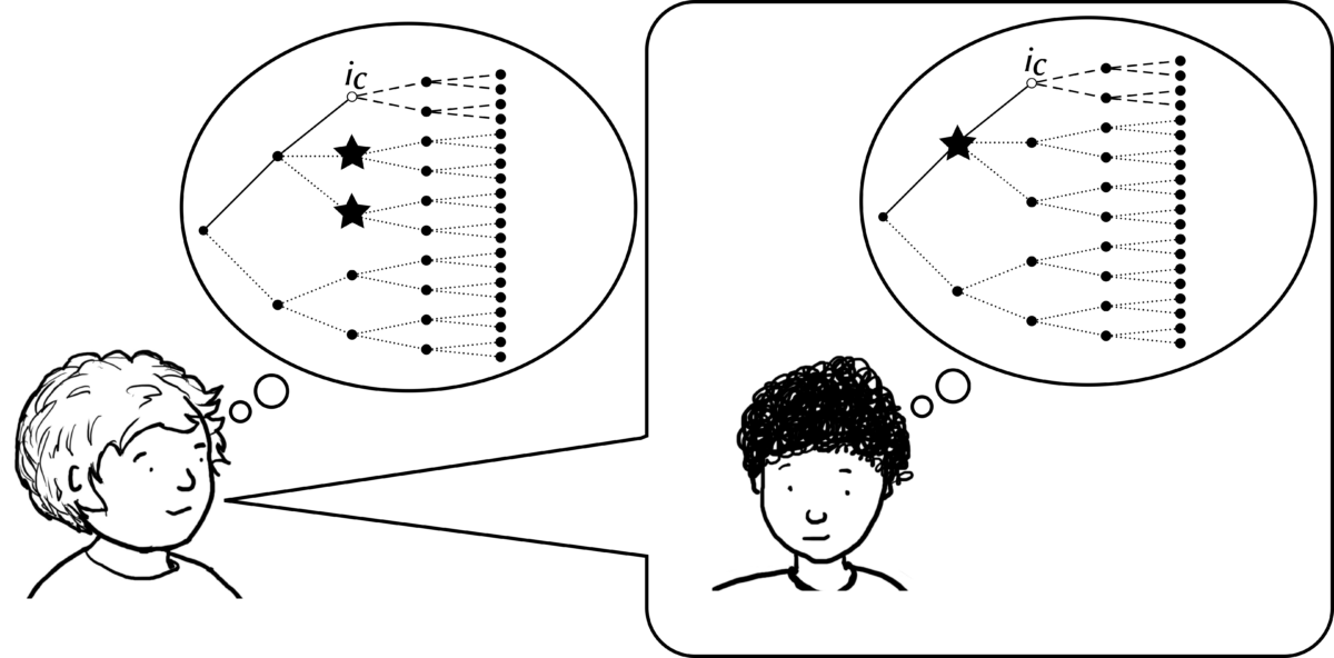
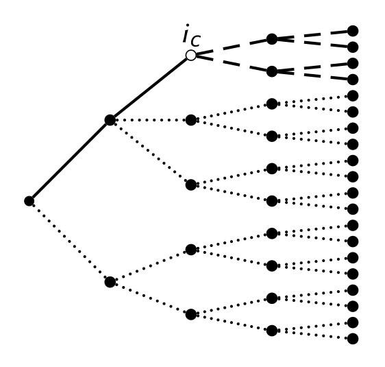
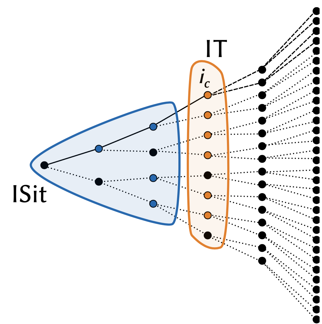
I was very happy to join a recent workshop on mistaken beliefs, organized by Simon Wimmer. I learned about intriguing new research by colleagues, and took the opportunity to present some ideas that relate contrafactivity to counterfactuality as expressed in natural languages. You can find my slides here.
Blog
Counterfactuality and mood
In my new paper, I take stock of cross-linguistically common functions and expressions of counterfactuality.
It also includes a discussion about whether expressions such as should encode counterfactuality or some kind of “weak” necessity.
You can download it here, or contact me.
Intro to morphology
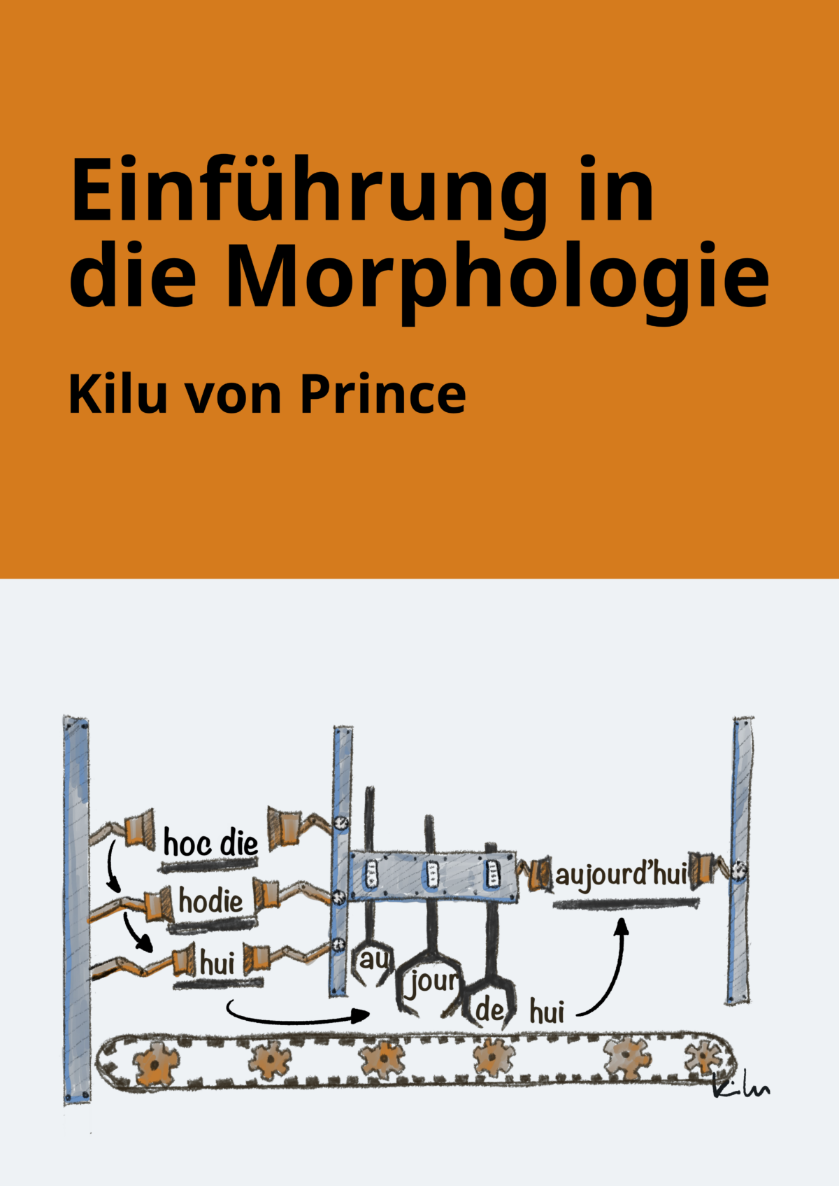
I just published my intro to morphology (Einführung in die Morphologie, in German). It starts out from the idea of the morphological cycle, which suggests that languages move through stages of isolating, agglutinating and fusional morphology, and uses this idea to introduce basic concepts of morphology, including inflection, derivation, paradigms, and different types and degrees of synthesis.
DGfS Workshop 2025
With my colleagues Ingo Plag and Jessica Nieder, we’re organizing a workshop on Morphological Variation at the upcoming DGfS in Mainz. I’m looking forward to reading the submitted abstracts!
Open Text Collections
I’m excited to be a regional editor for Open Text Collections! We’re aiming to publish curated, thematically consistent sets of interlinear glossed texts from a wide range of languages, and I’m looking forward to new submissions.
APLL 2024
Coming soon: Oceanic Word Units
My proposal for a project on Oceanic Word Units was recently approved by the German Research Society! We’ll start in 2024, but I’m already excited and looking forward to diving into vowel harmony, clitics, and the morphosyntax of subject markers. You can read the proposal here.
Afaka font
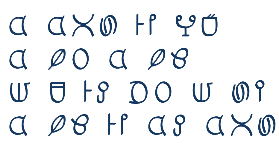
I regularly go a little overboard when designing puzzles for the German Olympiad of Linguistics, but for one of this year’s puzzles, I really outnerded myself. I designed a True Type Font for the writing system Afaka, which was developed for the creole language Ndyuka. It was conceived in 1910 by Afáka Atumisi and is named after its inventor. It’s a syllabary, partially based on a rebus system.

For example, the symbol representing the syllable /fo/ shows four vertical lines. And there is an Afaka word pronounced “fo”, which means “four” (yes, it’s cognate with the English word).
There is a preliminary Unicode sheet with codes, but the writing system hasn’t been fully developed and codified so far. Accordingly, my font is also only a preliminary solution to writing Ndyuka in Afaka script. But it’s great for playing around, and designing puzzles! You can download the font here.
Custom typological maps with R
I used to plot my typological language data to geo-spatial maps with Generic Mapping Tools, which is awesome, and where a simple two-liner will do the job. But I found this hard to use in teaching, since it doesn’t run smoothly on everyone’s operating system. So it’s time for me to move on and learn to do maps with R. There are a few awesome resources out there, including lingtypology, which reads data directly off glottolog.
But I wanted to plot data that is not included in a database, and since it’s actually easy, but not entirely trivial to find on the internet so far, here’s a short tutorial. First of all, here is our little data set, with geo-spatial coordinates for each language, language family and basic word order info. Save this to a text file in your working directory with the name “typology.txt”.
Language,Latitude,Longitude,Family,Family2,Word order
Movima,-13.81,-65.63,Isolate,9,0
Arapaho,43.39,-108.81,Algic,10,OV
Alta,15.69,121.45,Austronesian,12,OV
Savosavo,-9.13,159.81,Isolate,9,OV
Teop,-5.67,154.97,Austronesian,11,VO
Sumi,26,94.42,Sino-Tibetan,12,VO
Yali,-4.08,139.46,Nuclear-Trans-New-Guinea,13,OV
Beja,17.24,36.67,Afro-Asiatic,14,VO
Vera'a,-13.89,167.43,Austronesian,11,OV
Cabecar,9.67,-83.41,Chibchan,15,VO
Urum,42.04,43.99,Turkic,16,OV
Dolgan,71.11,94.29,Turkic,16,OV
Gorwaa,-4.24,35.8,Afro-Asiatic,14,OV
Pnar,24.82,92.26,Austroasiatic,17,0
Goemai,8.74,9.72,Afro-Asiatic,14,VO
English,53,-1,Indo-European,7,VO
Nung,-29.71,19.08,Tuu,18,VO
Bora,-2,-72.26,Boran,19,VSO
Nafsan,-17.7,168.38,Austronesian,11,OV
Komnzo,-8.65,141.52,Yam,20,OV
Kamas,55.07,94.83,Uralic,21,VO
Kakabe,10.6,-11.44,Mande,22,OV
Daakaka,-16.27,168.01,Austronesian,11,VO
Next in your R script, load the following packages. You might have to install them first:
library(ggplot2)
library(maps)
library(sf) #for advanced mapping options
library(viridisLite) #for pretty, color-blind friendly color palettes
Read in your map data and your language coordinates and save them to short variables like “map” and “df” (for data frame).
df <- read.csv("typology.txt")
head(df) #shows you the beginning of the data, good for trouble shooting
map <- map_data("world")
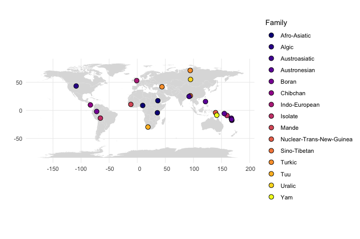
In order to plot your language coordinates with additional information about language families, do this:
#family
ggplot() +
  geom_polygon(data = map, aes(x = long, y = lat, group=group), fill="#dddddd") + #plots the world map in the background in light grey
  geom_point(data = df, aes(x = Longitude, y = Latitude, fill = factor(Family)), shape=21, size=3) + #plots the language coordinates
  theme_minimal()+ #fewer embellishments
  coord_sf()+ #nice proportions
  scale_fill_viridis_d(option = "plasma")+ #color scheme
  labs(fill = "Family", y="",x="") #labels
To get information about word order patterns, instead use this:
#word order
ggplot() +
  geom_polygon(data = map, aes(x = long, y = lat, group = group), fill="#dddddd") +
  geom_point(data = df, aes(x = Longitude, y = Latitude, fill = factor(Word.order)), shape=21,  size=3) +
  theme_minimal()+
  coord_sf()+
  scale_fill_viridis_d(option = "plasma")+
  labs(fill = "Word Order", y="",x="")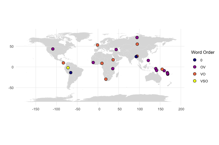
And since newbies sometimes use my tutorials: If you don’t understand something here, don’t give up, google it! Everyone does it, and most questions you might have, have already been asked and answered by someone somewhere.
Wrapping up 2022: more talks and publications
I haven’t been posting regularly about recent talks and publications, so here are a few more highlights from the second part of 2022:
- Colleagues and I published a paper on training RRG parsers on low resource languages, including Daakaka data.
- I gave a talk at the awesome linguistics department in Cologne, with a few more thoughts about wordhood in Daakaka.
- I was also invited to the phenomenal UT Texas (which curiously expands to University of Texas at Austin) department of linguistics, which combines two of my favourite subjects, linguistic fieldwork and formal semantics. This gave me a chance to get back to some of my ideas about modal semantics.

