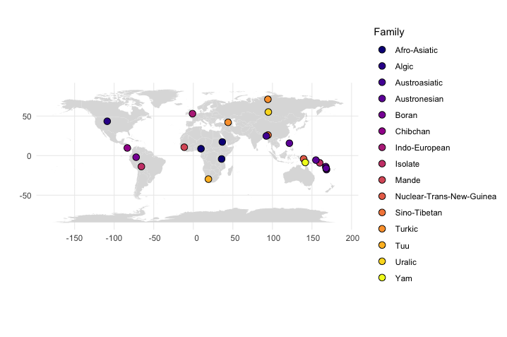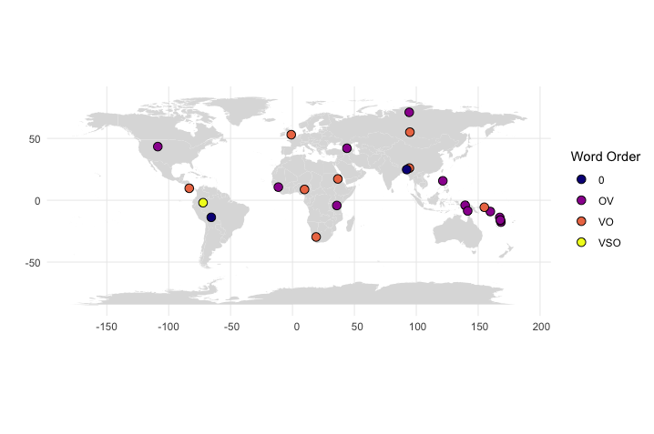
I made a tutorial on how to plot typological data (here from grambank) with R.
Edit: I redid the tutorial to reflect a more sustainable workflow, using the data as published on zenodo rather than the download link on grambank. I also added part 2 on how to combine two data sets.
Thanks go to Robert Forkel and Hedvig Skirgård, who were very helpful in pointing me to the right places and resources. Shout-out to Simon Greenhill for creating the rcldf package.
Here is the code.
# For any package on cran that you have not installed yet,
# RStudio will probably ask you whether you want to install.
# Otherwise, install the package with the command install.packages("PACKAGE"),
# do not forget the quotation marks. Example:
# install.packages("sf")
library(ggplot2)
library(dplyr)
library(sf)
library(rnaturalearth)
# the rnaturalearthhires package is not on cran,
# because it is too big. Uncomment to download package
 install.packages(
  "rnaturalearthhires",
  repos = "https://ropensci.r-universe.dev",
  type = "source"
)
library(rnaturalearthhires)

# The rcldf package is also not on cran, so you have to install it with devtools.
# Uncomment the following lines to install package.
# library(devtools)
# devtools::install_github("SimonGreenhill/rcldf", dependencies = TRUE)

library(rcldf)

# Check out the documentation here for exploring the rcldf package:
# https://github.com/grambank/grambank/wiki/Fetching-and-analysing-Grambank-data-with-R
# The following section is mostly taken from there.

grambank <-  rcldf::cldf(mdpath = "https://zenodo.org/records/7740140/files/grambank/grambank-v1.0.zip")
# what tables are there?
summary(grambank)

# get languages:
head(grambank$tables$LanguageTable)
# get values:
head(grambank$tables$ValueTable)

# the package also has a command to join various tables into one big table,
# so we can look up parameter values and coordinates in one data frame.
gb.wide <- as.cldf.wide(grambank, 'ValueTable')
head(gb.wide)

# Now we proceed with making our table for numeral classifiers in Cameroon
# (or the parameter and region of your choice)

# First, we create or map data for Cameroon:
cameroon <- ne_states(country = "Cameroon", returnclass = "sf")

# Now, we want to filter the grambank data.
# We only want language coordinates within Cameroon.

# We first need to figure out the map meta data for our country map.
st_crs(cameroon)
# The crucial part of the output here is this:
# Coordinate Reference System:
# User input: WGS 84
# See here for further reference:
# https://earthdatascience.org/courses/earth-analytics/spatial-data-r/understand-epsg-wkt-and-other-crs-definition-file-types/

# We can save this parameter like so:
projcrs <- "+proj=longlat +datum=WGS84 +no_defs +ellps=WGS84 +towgs84=0,0,0"
gbsf <- st_as_sf(x = gb.wide,
                      coords = c("Longitude", "Latitude"),
                      crs = projcrs, na.fail = FALSE)
# now we can filter our grambank table for those
# languages that are spoken in Cameroon
camergb <-  st_filter(gbsf, cameroon)
head(camergb)

# Next, we filter for the parameter we want to look at.
# In our example, that's numeral classifiers.
# We can look up its code at  https://grambank.clld.org/parameters
# The parameter for numeral classifiers is GB057.
camergb.clf <- filter(camergb, Parameter_ID == "GB057")

camergb.clf
# Here, we plot the Grambank data to a Map
ggplot() +
  geom_sf(data=cameroon, fill="#eeeeee")+
  geom_sf(data=camergb.clf, aes(fill=as.factor(Value)), shape=21)+
  scale_fill_manual(values=c("#ffaa99"), labels=c("absent", "unkown")) +
  labs(fill="Classifiers")+
  theme_void()


############################################
#     Part 2: Combine with second dataset  #
############################################

#Classifiers from Her et al.
heretal <- read.csv("https://raw.githubusercontent.com/cldf-datasets/wacl/refs/heads/main/raw/WACL_v1.csv")
head(heretal)
# Replace values to make them compatible with grambank values
heretal$CLF[heretal$CLF == FALSE] <- 0
heretal$CLF[heretal$CLF == TRUE] <- 1
heretal

# Transform data frame to shape file object
heretalSF <- st_as_sf(x = heretal,
                      coords = c("longitude", "latitude"),
                      crs = projcrs, na.fail = FALSE)

# Filter for Cameroonian languages
camerher <- st_filter(heretalSF, cameroon)
head(camerher)

# Combine dataframes camerher and camergb.clf into camerclf
# First, replace column name "Value" by "CLF" in the grambank data
# to conform with the other study
camergb.clf <- camergb.clf %>% rename_at('Value', ~'CLF')
# replace value "?" by "3" in grambank data.
# this will create a nicer order of categories later
camergb.clf <- camergb.clf |> mutate(CLF = ifelse(is.na(CLF), 3, CLF))
# currently, the grambank value is stored as a character string
# <chr>, because it originally contained "?"
# We want to store it as a number instead, for nicer automatic ordering
camergb.clf$CLF <- sapply(camergb.clf$CLF, as.double)
# Check if everything is fine.
View(camergb.clf)
# Add the camerher rows under the grambank rows.
# create an extra column "id" to index the data set
# id= 1 --> grambank, id = 2 --> Her et al.
camerclf <- bind_rows(list(camergb.clf, camerher), .id = "id")
camerclf

# Combine everything into one plot
ggplot() +
  geom_sf(data=cameroon, fill="#eeeeee")+
  geom_sf(data=camerclf, aes(shape=as.factor(id), fill=as.factor(CLF),  size=as.factor(id)))+
  scale_shape_manual(values=c(23,21), labels=c("Grambank", "Her et al. (2022)"))+
  scale_fill_manual(values=c("#ffaa99", "black", "white"), labels=c("absent", "present", "unkown")) +
  guides(fill=guide_legend(override.aes = list(shape=21)))+
  scale_size_manual(values=c(3,1.5), labels=c("Grambank", "Her et al. (2022)"))+
  labs(fill="Classifiers", shape="Dataset", size="Dataset")+
  theme_void()